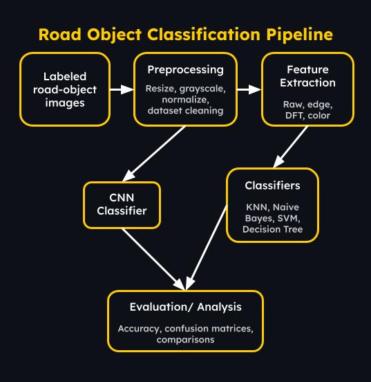
Baseline ML classifiers on dashcam footage — KNN, Naive Bayes, SVM, and Decision Tree tested across 2, 3, and 5+ object classes in MATLAB.
A compact summary of the project goal, classifier comparison, main result, and why the result matters for real-world driving image data.
Classify roadside objects from dashcam-style images using MATLAB image preprocessing and baseline machine-learning classifiers.
KNN, Naive Bayes, SVM, and Decision Tree models were trained and tested on labeled road-object image datasets.
SVM performed best on the refined real-world dataset, reaching about 91.4% accuracy on the car, pedestrian, and sign run.
The results show how dataset quality, class balance, and feature choices can change classifier performance as much as the model itself.
This report describes the results of running four MATLAB classifiers on labeled dashcam image datasets, evaluating differences in computation speed and accuracy: K Nearest Neighbors (KNN), Naive Bayes, Support Vector Machine (SVM), and Decision Tree.
All images were resized to a common resolution and converted into fixed-length grayscale pixel feature vectors. Datasets were balanced at 50 images per class for initial experiments.
Our project followed a full road-object image classification pipeline, which we later repeated after improving the realism and quality of the dataset. We began by gathering labeled object images and organizing them by class. Each image was resized to a common resolution and preprocessed through steps such as grayscale conversion, normalization, and data cleaning to make the inputs more consistent. We then compared multiple feature representations, including raw pixel values, edge-based features, frequency-domain features derived from the discrete Fourier transform, and color-based features. Using these representations, we trained and evaluated four MATLAB classifiers: KNN, Naive Bayes, SVM, and Decision Tree. Model performance was measured using confusion matrices, accuracy comparisons, and analysis across both balanced and refined real-world datasets. After finding that the original dataset contained unrealistic and suboptimal images, we replaced many of those examples with more representative dashcam-style objects and reran the classification pipeline to observe how dataset realism changed the results.
The image data was treated as a 2D signal: first prepared into a consistent form, then transformed into features that classifiers could compare.
Sobel-style edge filters were used to emphasize object boundaries and local intensity changes before classification.
Grayscale conversion and resizing standardized each image so every sample became a comparable fixed-length signal.
Frequency-domain features summarized how image energy was distributed across low, middle, and high spatial frequencies.
HOG and CNN-style features were considered as stronger learned or shape-aware feature options beyond the core DSP tools.
Each classifier needs a numerical feature vector, so the images were transformed into several representations before training.
Flattened grayscale image values provide a simple baseline representation.
Filtered edge magnitude and direction summarize object outlines.
FFT band-energy values describe frequency content in the image.
RGB histograms capture broad color distribution for traffic signs, cars, and pedestrians.
outside features can capture shape patterns or learned visual structure better than raw pixels alone.
Initially, we struggled finidng good datasets with cropped dash-cam images of the classes we desired.
So we used some suboptimal datasets while we procured and produced our own dataset.
We used labeled datasets from Kaggle and dashcam-related sources.
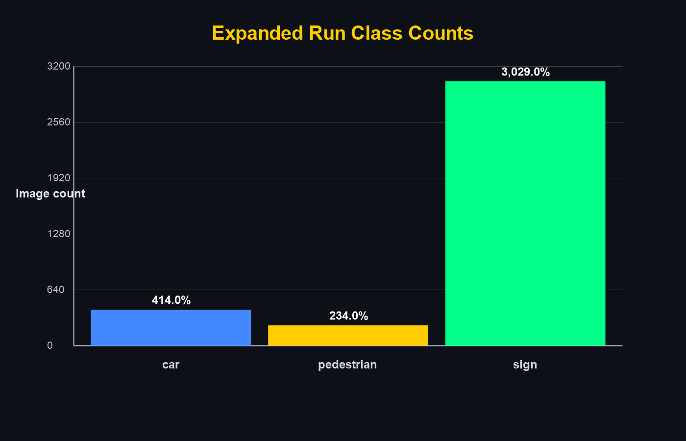
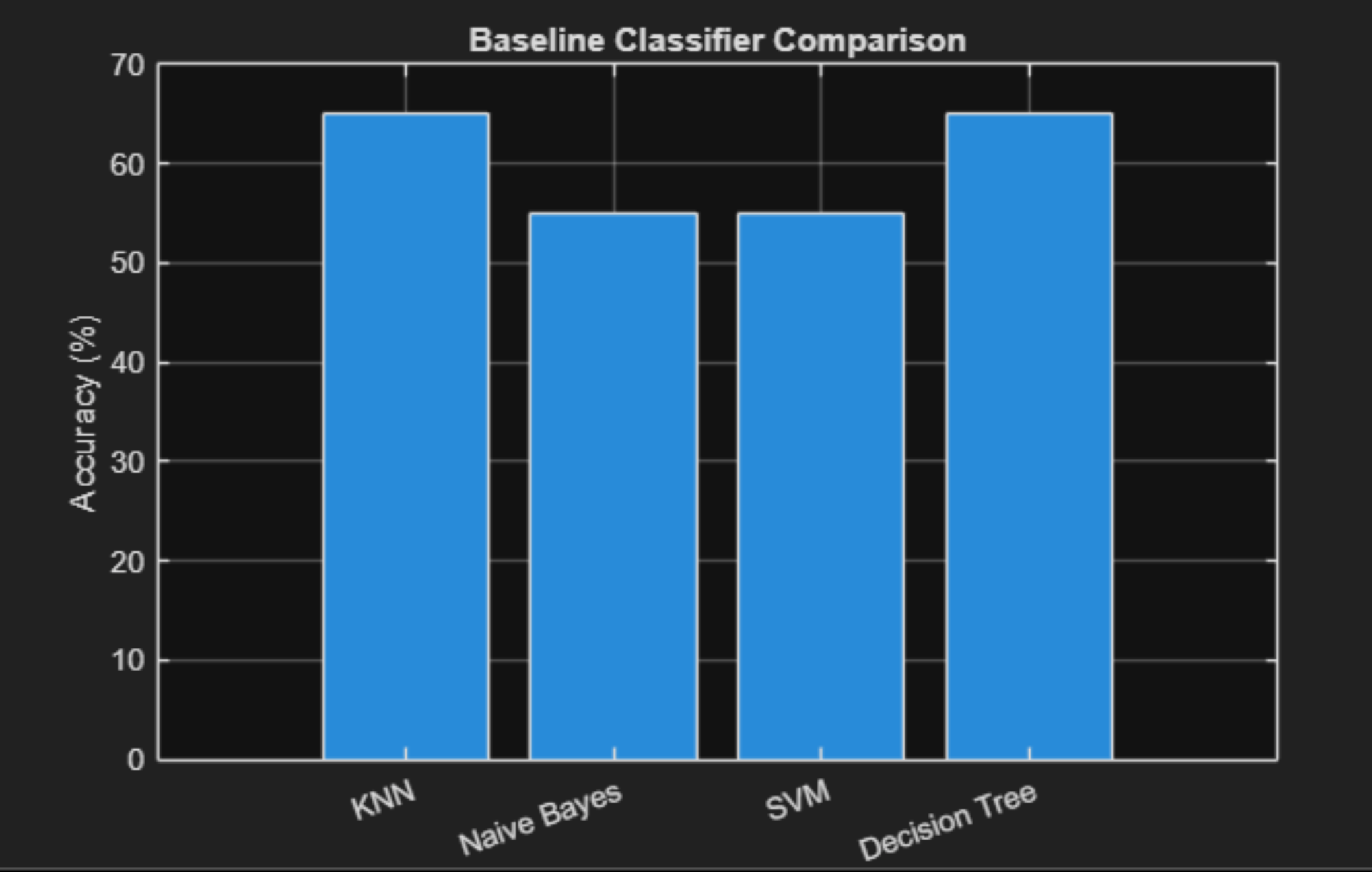
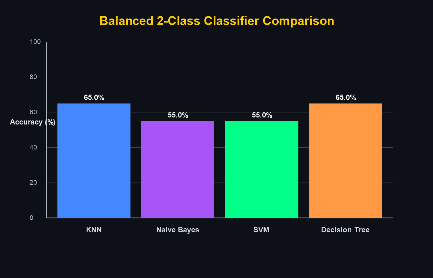
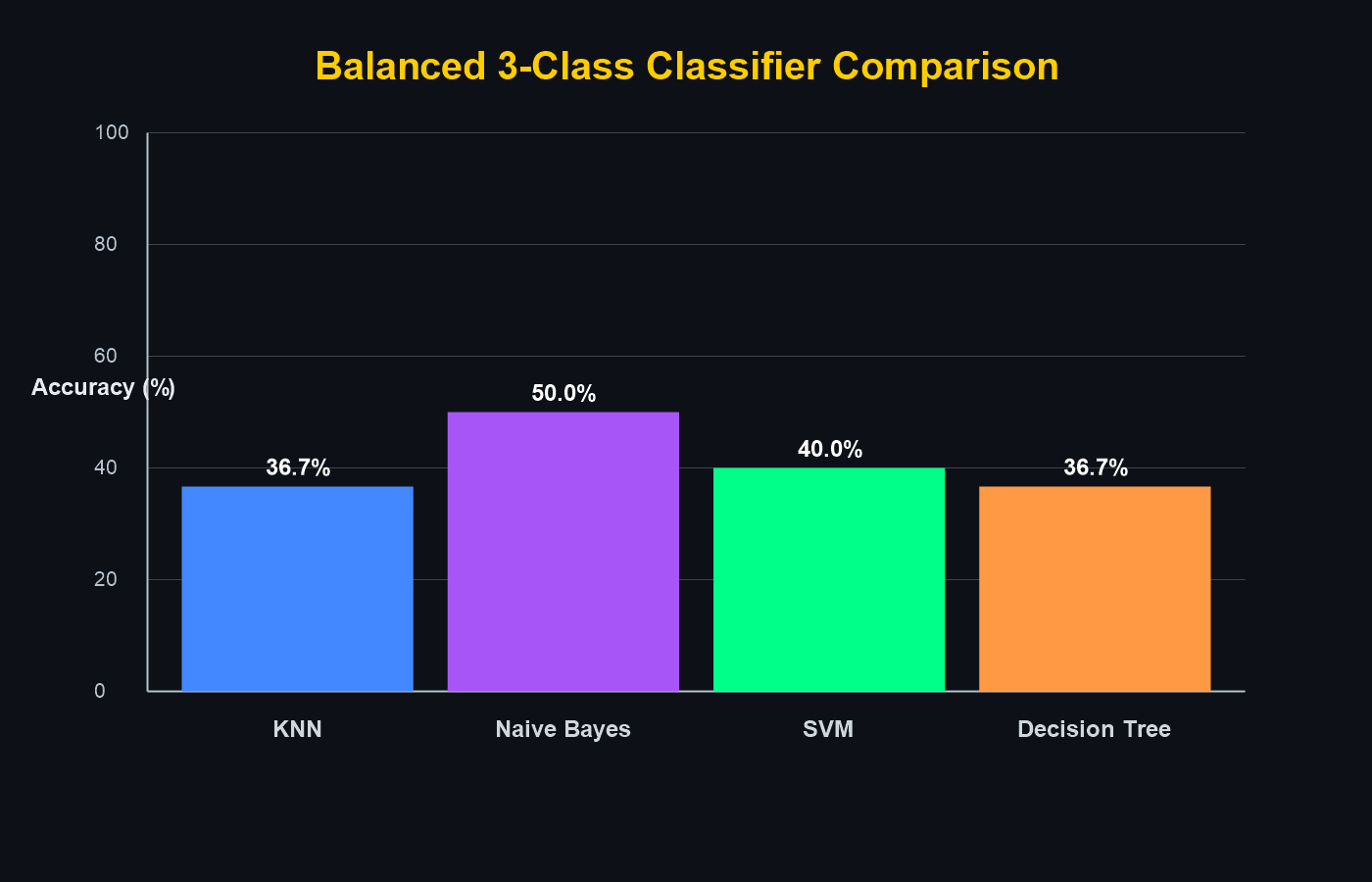
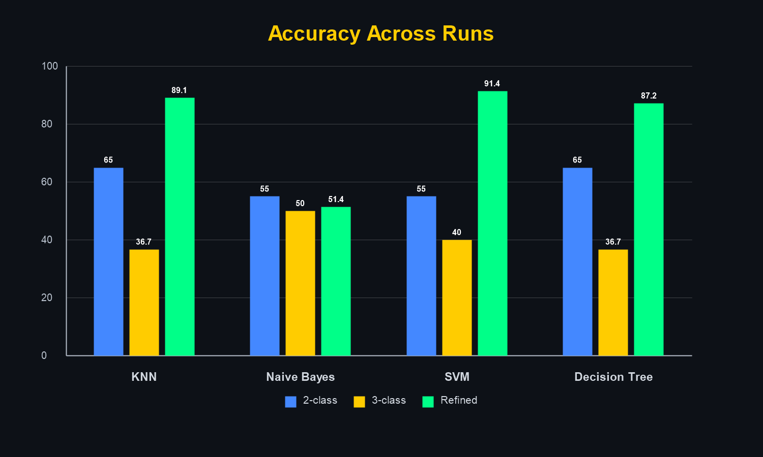
Initial experiments balanced all classes at 50 images each.
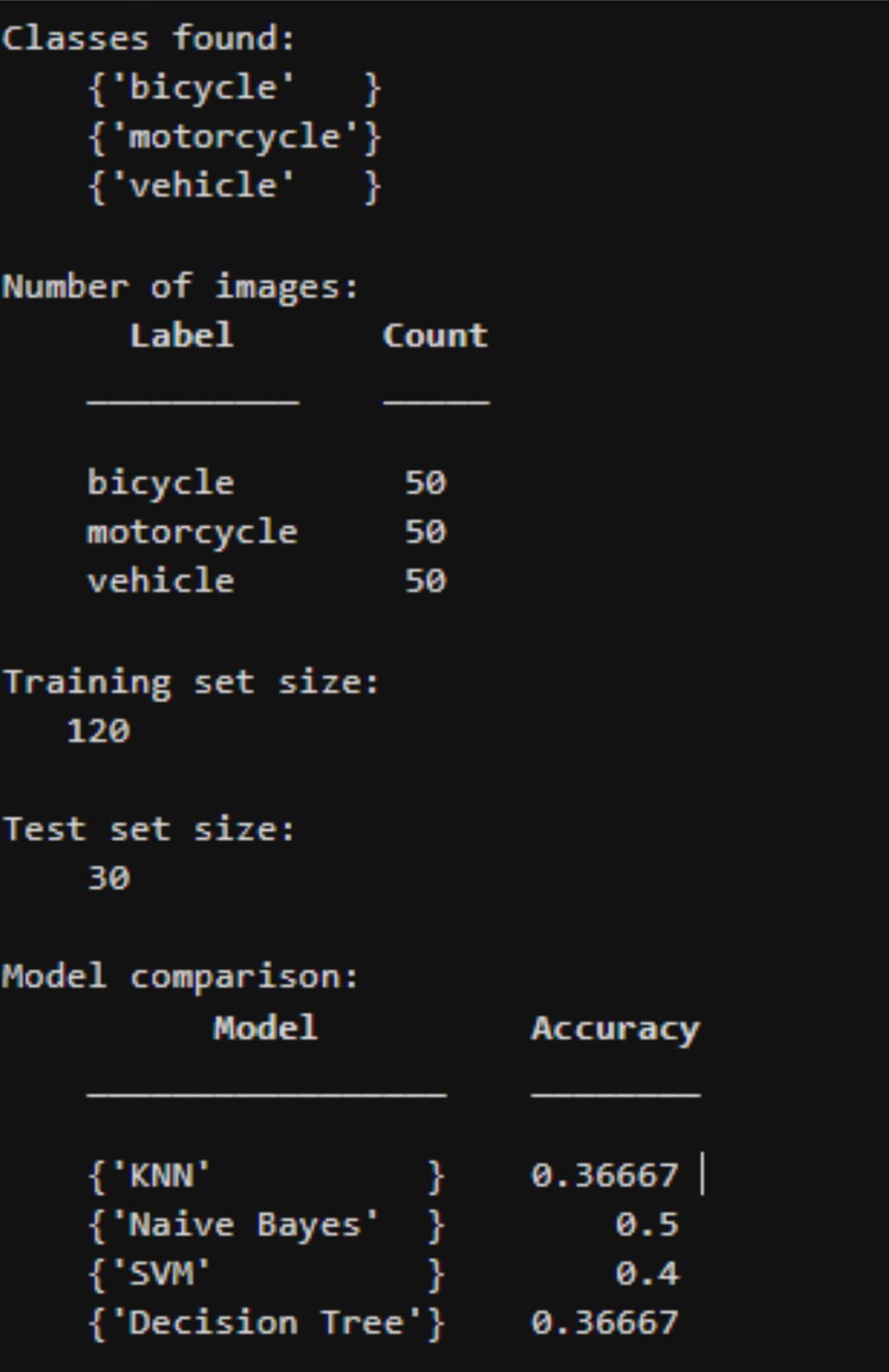
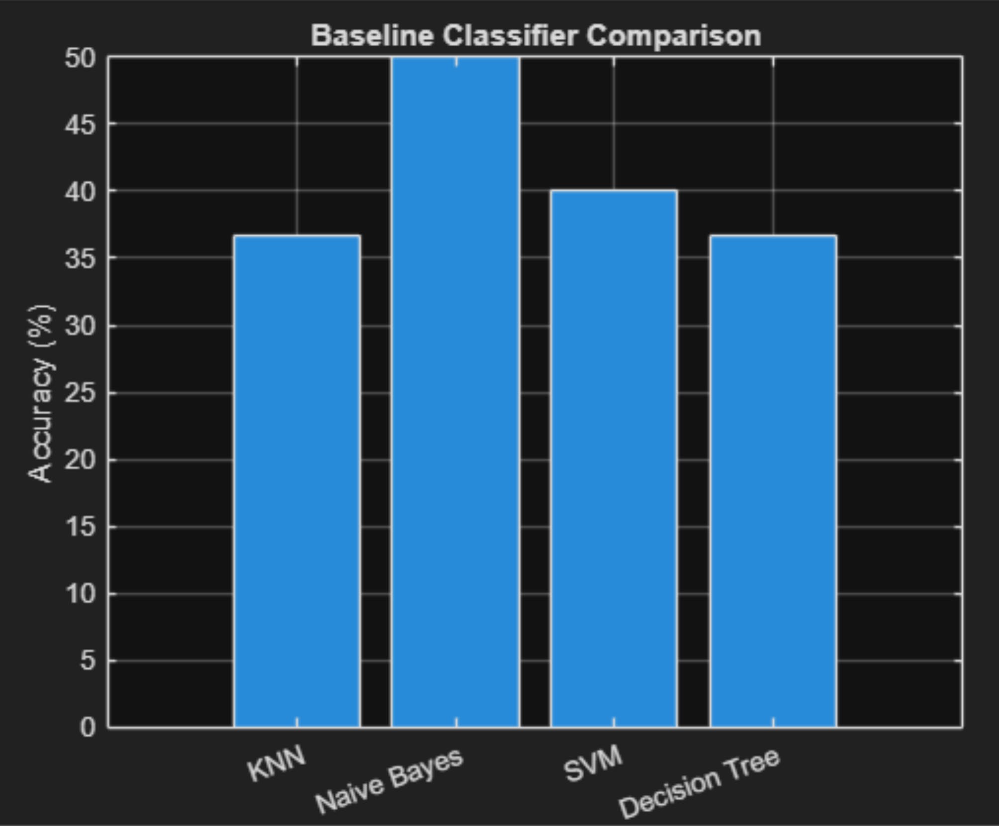
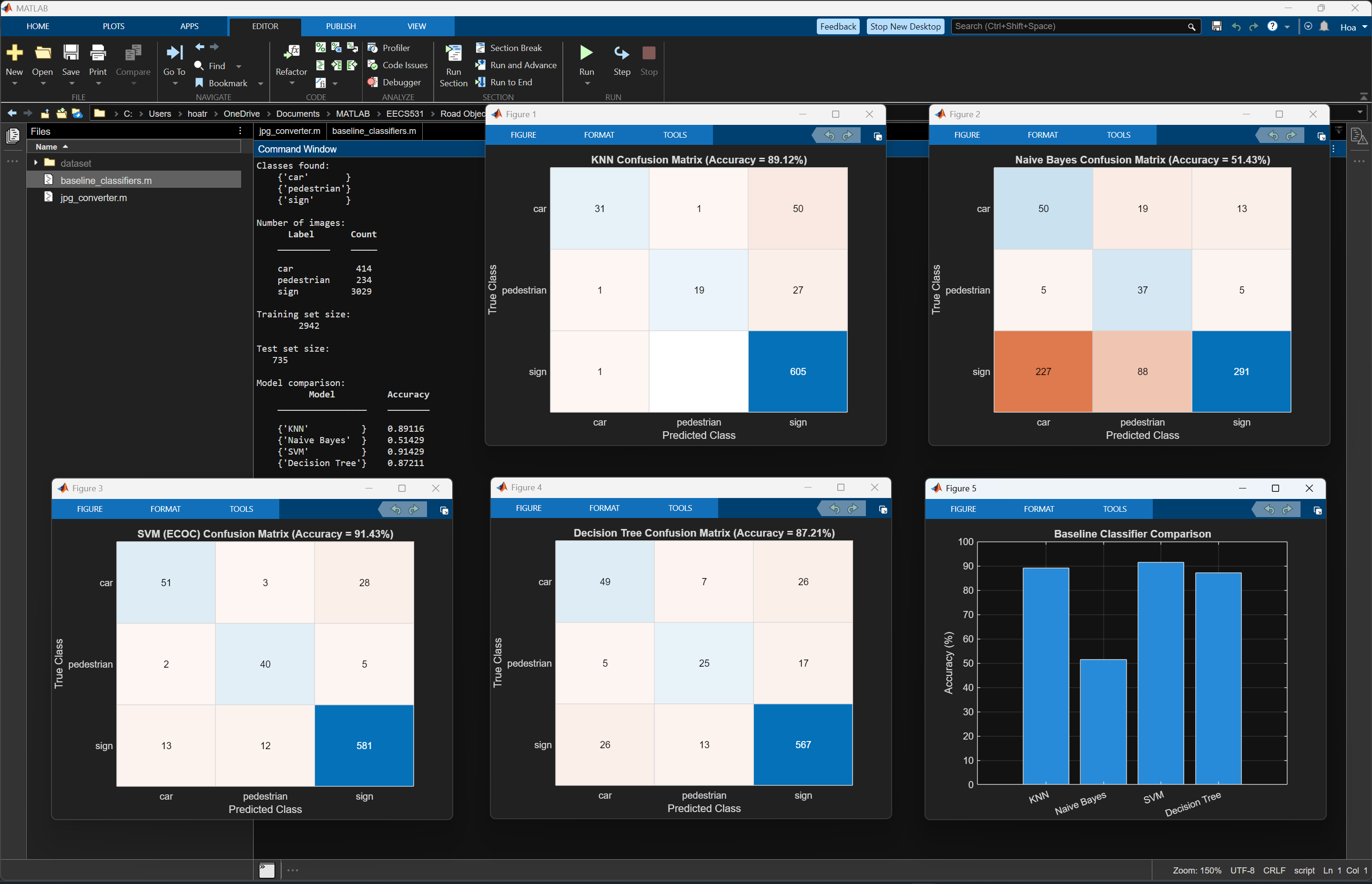
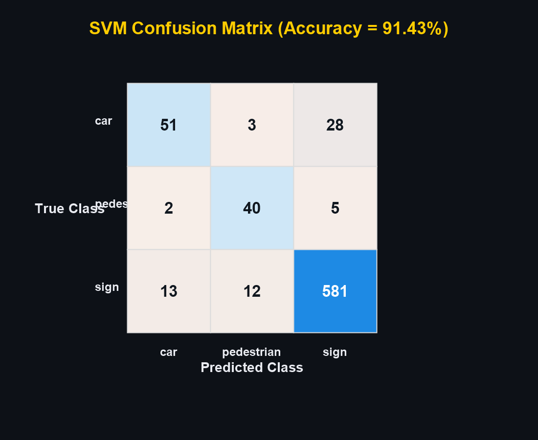
Later runs used unbalanced real-world proportions (e.g. 414 cars, 234 pedestrians, 3029 signs) to better reflect deployment conditions.
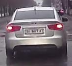
To improve realism, we moved away from an older car dataset after finding many images that were not representative of dashcam footage. It contained luxury vehicles (e.g., Rolls-Royces), heavily edited promotional images, text overlays, and staged settings. Using such images risks teaching the model non-generalizable patterns that would hurt roadside detection in practice. BadCar(43).jpg is an example of an image that triggered this refinement.
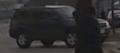
We created part of our own dataset by cropping objects from authentic dashcam footage, improving perspective, lighting, motion blur, and framing consistency. 
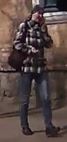
However, this custom set has limitations: many clips were sourced from Russia and fewer from the United States, Canada, and China. Pedestrian data may underrepresent demographic, clothing, and environment diversity in North America, which could produce uneven model performance across groups and regions. pedestrian46.jpg exemplifies this limitation. Expanding to broader demographic and geographic data is an important next step.
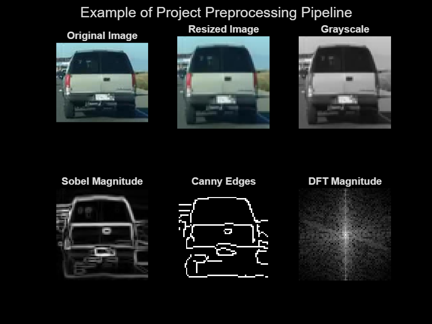
All images were in JPG format for their smaller file size and prevalence in real dashcam footage.
Actual MATLAB output charts from the 2-class and 3-class balanced runs (50 images per class). Accuracy decreases as more classes are added. Must disclaim that we initally used suboptimal datasets which included images that weren't fully cropped nor sourced from dashcam footage.
Train: 80 images | Test: 20 images
Train: 120 images | Test: 30 images
A new run with refined, unbalanced, real-world class proportions: 3 classes (car, pedestrian, sign)
with over 700 screenshots taken by us from real dashcam footage.
— Car: 414, Pedestrian: 234, Sign: 3,029. Training set: 2,942 · Test set: 735.
With a larger, refined, and unbalanced dataset that accurately reflects realworld data. Most classifiers perform dramatically better — especially SVM, which achieves over 91% accuracy. However, Naive Bayes performed significantly worse than any other classifier which revealed a fundamental flaw. That the Naive Bayes classifier will assign a prior probability based on how often a class appears in training sets.
⚠ Important caveat: Signs dominate at 3,029 images. High accuracy may reflect class imbalance rather than true model strength. Naive Bayes drops to 51% — it struggles with imbalanced distributions.
SVM is the clear winner at 91.43%, consistent with literature suggesting SVM handles high-dimensional pixel features well. The jump from 55% → 91% from balanced-50 to the real dataset underscores how data volume dramatically impacts baseline classifiers. Naive Bayes remains the weakest, sensitive to class imbalance.
Turay, T. & Vladimirova, T. "Toward performing image classification and object detection with CNNs in autonomous driving systems: A survey." IEEE Access, vol. 10, pp. 14076–14119, 2022.
The main script is run_demo.m. It loads the included sample dataset, preprocesses each image, extracts selected features, trains the four classifiers, and displays confusion matrices plus an accuracy comparison chart.
A small sample dataset is included in dataset_sample/ so the demo can run from the project zip. The full development dataset and MATLAB project files are hosted separately in the Google Drive file Road_Object_Classification.zip.
The website summarizes the project story and results, while the MATLAB files provide the reproducible classifier pipeline used for the sample run.
Submitted March 22, 2026 · Umich
Helped source and clean datasets, compare classifier results, and interpret the improved real-world run.
Worked on MATLAB classifier coding, confusion-matrix evaluation, and result analysis across model runs.
Contributed to dataset review, report writing, and the paper summary connecting the work to autonomous-driving literature.
Built and refined the website design, organized the visual results, and connected the code outputs to the web report.
Supported feature-extraction experiments, dataset preparation, and analysis of strengths, weaknesses, and future improvements.